# civilytics
Brand themes, color palettes, and utility functions for [Civilytics
Consulting](https://www.civilytics.com). The package provides a complete
ggplot2 theme system drawn from the Civilytics design system — warm
paper backgrounds, civic-navy ink, and editorial typography — along with
10 curated color palettes, logo composition helpers, and data-wrangling
utilities for public-sector analysis.
## Installation
Install from the Civilytics Gitea server:
``` r
# install.packages("remotes")
remotes::install_git("https://gitea.civilytics.org/Civilytics/civilyticsR.git")
```
## Quick start
``` r
library(civilytics)
library(ggplot2)
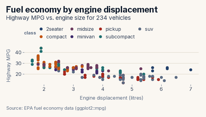
ggplot(mpg, aes(displ, hwy, colour = class)) +
geom_point(size = 2.5) +
scale_color_civilytics() +
labs(
title = "Fuel economy by engine displacement",
subtitle = "Highway MPG vs. engine size for 234 vehicles",
caption = "Source: EPA fuel economy data (ggplot2::mpg)",
x = "Engine displacement (litres)",
y = "Highway MPG"
) +
theme_civilytics()
```
 ## Color palettes
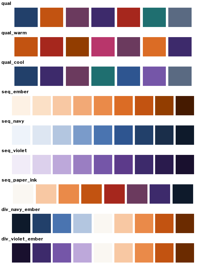
The package ships 53 named brand colors in `civilytics_colors` and 10
curated palettes in `civilytics_palettes`. Use `civilytics_palette()` to
retrieve colors by name, or pass palettes directly to the ggplot2
scales.
### Palette gallery
## Color palettes
The package ships 53 named brand colors in `civilytics_colors` and 10
curated palettes in `civilytics_palettes`. Use `civilytics_palette()` to
retrieve colors by name, or pass palettes directly to the ggplot2
scales.
### Palette gallery
 ### Using palettes
``` r
# Discrete fill with the qualitative palette
ggplot(mpg, aes(class, fill = class)) +
geom_bar(show.legend = FALSE) +
scale_fill_civilytics() +
labs(title = "Vehicle counts by class", x = NULL, y = NULL) +
theme_civilytics(grid = "y")
```
### Using palettes
``` r
# Discrete fill with the qualitative palette
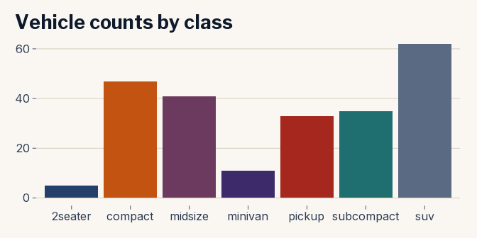
ggplot(mpg, aes(class, fill = class)) +
geom_bar(show.legend = FALSE) +
scale_fill_civilytics() +
labs(title = "Vehicle counts by class", x = NULL, y = NULL) +
theme_civilytics(grid = "y")
```
 ``` r
# Continuous fill with a sequential palette
ggplot(faithfuld, aes(waiting, eruptions, fill = density)) +
geom_tile() +
scale_fill_civilytics("seq_ember", discrete = FALSE) +
labs(title = "Old Faithful eruption density") +
theme_civilytics(grid = "none")
```
``` r
# Continuous fill with a sequential palette
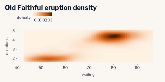
ggplot(faithfuld, aes(waiting, eruptions, fill = density)) +
geom_tile() +
scale_fill_civilytics("seq_ember", discrete = FALSE) +
labs(title = "Old Faithful eruption density") +
theme_civilytics(grid = "none")
```
 ## Themes
Three theme variants cover the most common output contexts. All share
the same typographic structure and accept `grid` and `paper_bg`
parameters.
### Editorial (default)
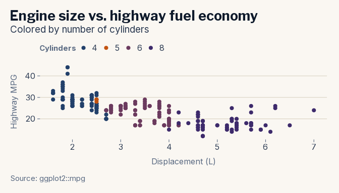
The default theme uses a warm paper background with horizontal gridlines
— an editorial, Pew-style layout.
``` r
base_plot <- ggplot(mpg, aes(displ, hwy)) +
geom_point(aes(colour = factor(cyl)), size = 2) +
scale_color_civilytics() +
labs(
title = "Engine size vs. highway fuel economy",
subtitle = "Colored by number of cylinders",
caption = "Source: ggplot2::mpg",
colour = "Cylinders",
x = "Displacement (L)", y = "Highway MPG"
)
base_plot + theme_civilytics()
```
## Themes
Three theme variants cover the most common output contexts. All share
the same typographic structure and accept `grid` and `paper_bg`
parameters.
### Editorial (default)
The default theme uses a warm paper background with horizontal gridlines
— an editorial, Pew-style layout.
``` r
base_plot <- ggplot(mpg, aes(displ, hwy)) +
geom_point(aes(colour = factor(cyl)), size = 2) +
scale_color_civilytics() +
labs(
title = "Engine size vs. highway fuel economy",
subtitle = "Colored by number of cylinders",
caption = "Source: ggplot2::mpg",
colour = "Cylinders",
x = "Displacement (L)", y = "Highway MPG"
)
base_plot + theme_civilytics()
```
 ### Grid options
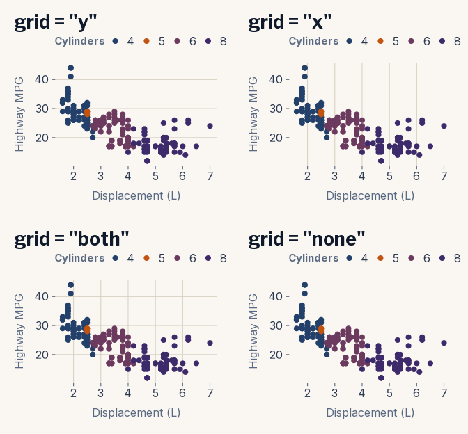
The `grid` parameter controls which major gridlines are drawn.
### Grid options
The `grid` parameter controls which major gridlines are drawn.
 ### Dark
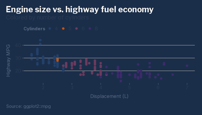
Dark navy background with light text, suitable for presentations or
dashboards on dark surfaces.
``` r
base_plot + theme_civilytics_dark()
```
### Dark
Dark navy background with light text, suitable for presentations or
dashboards on dark surfaces.
``` r
base_plot + theme_civilytics_dark()
```
 ### Slide
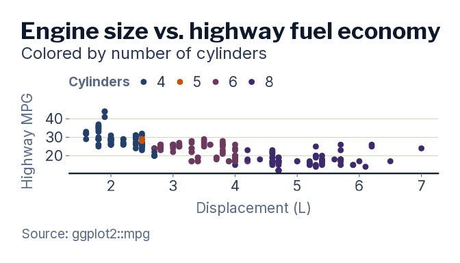
Transparent background and larger base font (18 pt), sized for Reveal.js
slides or PowerPoint exports.
``` r
base_plot + theme_civilytics_slide()
```
### Slide
Transparent background and larger base font (18 pt), sized for Reveal.js
slides or PowerPoint exports.
``` r
base_plot + theme_civilytics_slide()
```
 ### Facets
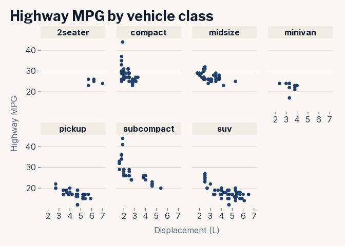
Facet strips use the `paper_2` tint, with the title font.
``` r
ggplot(mpg, aes(displ, hwy)) +
geom_point(colour = civilytics_colors["navy_600"], size = 1.5) +
facet_wrap(~class, ncol = 4) +
labs(
title = "Highway MPG by vehicle class",
x = "Displacement (L)", y = "Highway MPG"
) +
theme_civilytics(grid = "y")
```
### Facets
Facet strips use the `paper_2` tint, with the title font.
``` r
ggplot(mpg, aes(displ, hwy)) +
geom_point(colour = civilytics_colors["navy_600"], size = 1.5) +
facet_wrap(~class, ncol = 4) +
labs(
title = "Highway MPG by vehicle class",
x = "Displacement (L)", y = "Highway MPG"
) +
theme_civilytics(grid = "y")
```
 ## Logo utilities
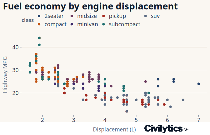
Add the Civilytics logo to any ggplot using the pipe-friendly
`civilytics_logo()` or the lower-level `add_logo()` /
`make_logo_grob()`. The logo is automatically right-aligned below the
plot area. Wrap the ggplot chain in parentheses before piping — R’s `|>`
binds tighter than `+`.
### Wordmark on a light plot
``` r
p <- ggplot(mpg, aes(displ, hwy, colour = class)) +
geom_point(size = 2) +
scale_color_civilytics() +
labs(
title = "Fuel economy by engine displacement",
caption = "Source: EPA fuel economy data (ggplot2::mpg)",
x = "Displacement (L)", y = "Highway MPG"
) +
theme_civilytics()
grid::grid.draw(civilytics_logo(p))
```
## Logo utilities
Add the Civilytics logo to any ggplot using the pipe-friendly
`civilytics_logo()` or the lower-level `add_logo()` /
`make_logo_grob()`. The logo is automatically right-aligned below the
plot area. Wrap the ggplot chain in parentheses before piping — R’s `|>`
binds tighter than `+`.
### Wordmark on a light plot
``` r
p <- ggplot(mpg, aes(displ, hwy, colour = class)) +
geom_point(size = 2) +
scale_color_civilytics() +
labs(
title = "Fuel economy by engine displacement",
caption = "Source: EPA fuel economy data (ggplot2::mpg)",
x = "Displacement (L)", y = "Highway MPG"
) +
theme_civilytics()
grid::grid.draw(civilytics_logo(p))
```
 ### Compact mark
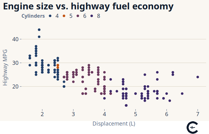
Use `type = "mark"` for the compact C-pulse icon instead of the full
wordmark.
``` r
p2_logo <- ggplot(mpg, aes(displ, hwy, colour = factor(cyl))) +
geom_point(size = 2) +
scale_color_civilytics() +
labs(
title = "Engine size vs. highway fuel economy",
colour = "Cylinders",
x = "Displacement (L)", y = "Highway MPG"
) +
theme_civilytics()
grid::grid.draw(civilytics_logo(p2_logo, type = "mark"))
```
### Compact mark
Use `type = "mark"` for the compact C-pulse icon instead of the full
wordmark.
``` r
p2_logo <- ggplot(mpg, aes(displ, hwy, colour = factor(cyl))) +
geom_point(size = 2) +
scale_color_civilytics() +
labs(
title = "Engine size vs. highway fuel economy",
colour = "Cylinders",
x = "Displacement (L)", y = "Highway MPG"
) +
theme_civilytics()
grid::grid.draw(civilytics_logo(p2_logo, type = "mark"))
```
 ### Multi-plot layout with logo
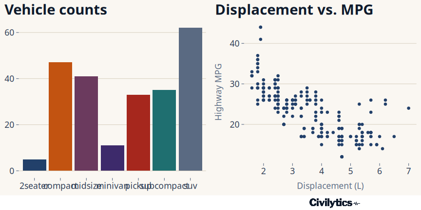
Use `add_logo_ga()` to attach a single logo below a row of plots.
``` r
p1 <- ggplot(mpg, aes(class, fill = class)) +
geom_bar(show.legend = FALSE) +
scale_fill_civilytics() +
labs(title = "Vehicle counts", x = NULL, y = NULL) +
theme_civilytics(grid = "y")
p2 <- ggplot(mpg, aes(displ, hwy)) +
geom_point(colour = civilytics_colors["navy_600"], size = 1.5) +
labs(title = "Displacement vs. MPG", x = "Displacement (L)", y = "Highway MPG") +
theme_civilytics(grid = "y")
logo <- make_logo_grob()
grid::grid.draw(add_logo_ga(list(p1, p2), logo))
```
### Multi-plot layout with logo
Use `add_logo_ga()` to attach a single logo below a row of plots.
``` r
p1 <- ggplot(mpg, aes(class, fill = class)) +
geom_bar(show.legend = FALSE) +
scale_fill_civilytics() +
labs(title = "Vehicle counts", x = NULL, y = NULL) +
theme_civilytics(grid = "y")
p2 <- ggplot(mpg, aes(displ, hwy)) +
geom_point(colour = civilytics_colors["navy_600"], size = 1.5) +
labs(title = "Displacement vs. MPG", x = "Displacement (L)", y = "Highway MPG") +
theme_civilytics(grid = "y")
logo <- make_logo_grob()
grid::grid.draw(add_logo_ga(list(p1, p2), logo))
```
 ## Other utilities
The package also includes helpers for public-sector data analysis:
| Function | Purpose |
|:---|:---|
| `pretty_count()` / `pretty_per()` | Format numbers and percentages |
| `grade_level_to_num()` | Convert grade labels (KG, 01–12) to numeric |
| `race_short_names()` | Standardize NCES race/ethnicity categories |
| `get_fips()` / `get_stabbr()` | State FIPS code lookups |
| `clopper_pearson()` / `agresti_coull_interval()` | Proportion confidence intervals |
| `match_test()` / `trunc_match()` | Fuzzy join diagnostics |
| `perturb_count()` / `random_round()` | Privacy-preserving data perturbation |
## Maintaining brand assets
Logo and brand mark files live in `inst/img/`. The package ships both
PNG (for ggplot2 raster composition) and SVG (for Quarto/HTML output)
variants:
| File | Format | Used by |
|:---|:---|:---|
| `civilytics-wordmark.png` / `.svg` | Full “Civilytics” lockup | `make_logo_grob("wordmark", "light")`, Quarto templates |
| `civilytics-wordmark-reverse.png` / `.svg` | Light-on-dark wordmark | `make_logo_grob("wordmark", "dark")`, dark slides |
| `civilytics-mark.png` / `.svg` | Compact C-pulse icon | `make_logo_grob("mark", "light")` |
| `civilytics-mark-reverse.svg` | Light-on-dark mark | `make_logo_grob("mark", "dark")` |
| `civilytics-pulse.svg` | Standalone waveform glyph | Quarto slide footer chrome |
To update the logos, replace the files in `inst/img/` with new versions
using the same filenames. The PNG files must be raster images (the
ggplot2 logo functions read them via `png::readPNG()`). SVG files are
passed through as-is by Quarto and HTML templates.
After replacing files, re-render the README gallery to update the
screenshots:
``` r
devtools::load_all()
rmarkdown::render("README.Rmd")
```
## Other utilities
The package also includes helpers for public-sector data analysis:
| Function | Purpose |
|:---|:---|
| `pretty_count()` / `pretty_per()` | Format numbers and percentages |
| `grade_level_to_num()` | Convert grade labels (KG, 01–12) to numeric |
| `race_short_names()` | Standardize NCES race/ethnicity categories |
| `get_fips()` / `get_stabbr()` | State FIPS code lookups |
| `clopper_pearson()` / `agresti_coull_interval()` | Proportion confidence intervals |
| `match_test()` / `trunc_match()` | Fuzzy join diagnostics |
| `perturb_count()` / `random_round()` | Privacy-preserving data perturbation |
## Maintaining brand assets
Logo and brand mark files live in `inst/img/`. The package ships both
PNG (for ggplot2 raster composition) and SVG (for Quarto/HTML output)
variants:
| File | Format | Used by |
|:---|:---|:---|
| `civilytics-wordmark.png` / `.svg` | Full “Civilytics” lockup | `make_logo_grob("wordmark", "light")`, Quarto templates |
| `civilytics-wordmark-reverse.png` / `.svg` | Light-on-dark wordmark | `make_logo_grob("wordmark", "dark")`, dark slides |
| `civilytics-mark.png` / `.svg` | Compact C-pulse icon | `make_logo_grob("mark", "light")` |
| `civilytics-mark-reverse.svg` | Light-on-dark mark | `make_logo_grob("mark", "dark")` |
| `civilytics-pulse.svg` | Standalone waveform glyph | Quarto slide footer chrome |
To update the logos, replace the files in `inst/img/` with new versions
using the same filenames. The PNG files must be raster images (the
ggplot2 logo functions read them via `png::readPNG()`). SVG files are
passed through as-is by Quarto and HTML templates.
After replacing files, re-render the README gallery to update the
screenshots:
``` r
devtools::load_all()
rmarkdown::render("README.Rmd")
```